Does 85% Confidence Mean 85% Correct? Calibrating a Decision Model on a 12 GB Laptop GPU

Every decision API worth the name makes the same promise: when it says 85 %, it means 85 %. That number is the whole product. Chat models can fake it — ask a language model "how confident are you?" and it will produce a plausible-sounding figure with no statistical backbone. A decision model does something stricter: it reads a question and a fixed set of options, scores them in a single forward pass, and returns probabilities you can plug into a planner.

The open implementations of this idea (the Jev-style ecosystem: fastjev, jev-local, the DIY variants) all reduce to one mechanism — read the logits of the answer tokens instead of generating free text. That makes them cheap, deterministic, and auditable: you can check whether the probabilities are honest. So we checked.

We ran a 12 B open-weights model on an RTX 4080 Laptop (12 GB), fully local, through a 100-decision evaluation with a calibration phase and a self-repair loop. The headline findings:

Phase	Accuracy	Mean confidence	ECE
R0 — raw logits	70 %	83.4 %	0.137
R1 — temperature-calibrated	70 %	63.0 %	0.160
R2 — blind self-repair	82 %	63.5 %	0.190
R3 — told the answer	100 %	72.7 %	0.273

Raw overconfidence by 13 points. Temperature scaling deflates confidence almost to where accuracy lives — but doesn't reliably improve expected calibration error out of sample. And a single blind repair round, where the model is told only "you were wrong, look again", fixes 40 % of its misses. All numbers below are real runs on the laptop GPU.

The setup

No cloud, no API keys, one machine:

Component	Choice
GPU	RTX 4080 Laptop, 12 GB VRAM
Runtime	llama.cpp b11538 (CUDA), server on 127.0.0.1:8080
Model	Gemma-4-12B-IT, QAT Q4_0 GGUF (~7 GB, fits fully offloaded)
Decision harness	graphwiz-jev scripts — option logprobs via /completion with n_probs: 100
Calibration	single-temperature fit, minimising NLL on the training split
Evaluation	100 held-out CommonsenseQA-style everyday decisions, five options each

Why a 12 B general instruct model rather than a packaged decision stack such as fastjev? Because the point of this evaluation is the mechanism, not the product: option logits in, calibrated probabilities out — a recipe that works with any open-weights model llama.cpp can serve, and one you can audit line by line.

The pipeline is deliberately boring. For each decision, we render a prompt with the five options labelled A–E, close the model's thinking channel so it answers directly, request exactly one token with the top-100 logprob distribution, and read off the log-probability of each letter (impossible letters get −∞, floored at −30 nats to keep the softmax finite). Softmax over five numbers — that's the entire decision layer:

log_probs = option_logprobs(prompt)          # 5 nats from one forward pass
scaled    = [max(lp, FLOOR) / temperature for lp in log_probs]
probs     = softmax(scaled)
choice    = argmax(probs)

Because it is one forward pass per decision, the whole 100-question evaluation takes minutes, and the same prompt always yields the same probabilities. No sampling, no temperature-creativity tricks — the temperature here is purely a calibration dial.

The plumbing also exists as a tiny HTTP decision endpoint (POST /decide, returning raw and calibrated probabilities per option), which is how we wire the model into our ops agent — more on that at the end.

The architecture: a decision layer, not a model

"Decision model" sounds like a special network. It isn't — and that is the interesting part. Open up the packaged offerings — fastjev (a 4 B Qwen served over llama.cpp, vLLM, MLX or WebGPU), jev-local (9 B), the kev range (0.6–8 B), or the 27 B OpenJev (B300-class hardware only) — and the same three separable layers recur:

Layer	What it does	Artifact
1 · Constrained readout	one forward pass; letter-token logits; no generation loop, no sampling	prompt template + logprob readout
2 · Calibration	divides logits by a fitted scalar; fixes the confidence scale	temperature.json (ours: T = 2.44)
3 · Decision contract	fixed option set in, probabilities out; verbs: choice, boolean, score	the API shape

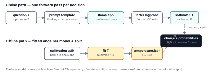
Three properties fall out of that shape, and each one matters operationally:

Latency is one prefill. No autoregressive loop means a decision costs the same as classifying one token — the entire 100-question evaluation in this article ran in minutes on a laptop GPU, and a server-grade deployment would handle thousands of decisions per minute per GPU.

The layer is separable from the model. We served a 12 B Gemma; the same template-readout-softmax recipe works with any instruct model llama.cpp can load. One caveat we verified the hard way: the temperature is a property of model + calibration split, not of the architecture. Swap the base model and you must re-fit T — but that is one pass over a few hundred decisions, not a training run.

Everything is auditable. A chat model's confidence is a sentence it made up. Here, every probability traces back to a logprob you can print, and the calibration artifact is a single number with a recorded provenance (split, loss, fit date). When a regulator or an operator asks "why 85 %?", there is an answer that isn't vibes.

R0: the raw model lies by 13 points

Untransformed, the model gets 70 % of the 100 decisions right while claiming an average of 83.4 % confidence. Expected calibration error (ECE, 15 bins) lands at 0.137 — but the aggregate hides where the dishonesty actually lives. The reliability table tells the real story (populated bins, three of ten shown):

Confidence bin	n	Mean confidence	Accuracy
0.93–1.00	49	0.982	0.878
0.87–0.93	13	0.904	0.692
0.53–0.60	6	0.569	0.500

Half the evaluation sits in the top bin, claiming 98 % confidence while being right 88 % of the time. That is the overconfidence cliff: when a raw LLM has basically decided, it reports decided, not probably. Six items in that top bin are wrong — and every one of them is wrong at 98 %+ confidence, the worst place for a decision consumer to inherit an error.

This is exactly the pathology that motivated hosted decision models in the first place. A planner consuming these probabilities would escalate aggressively on phantom certainties.

R1: temperature fixes the cliff — mostly

The classic fix is one scalar. Fit a temperature T on a held-out calibration split by minimising negative log-likelihood, then divide all logits by T before the softmax. Our fit lands at T = 2.44 — comfortably above 1.0, confirming systematic overconfidence.

The repair works where the problem was (same format; the last row is the low tail that matters later):

Confidence bin	n	Mean confidence	Accuracy
0.93–1.00	11	0.973	1.000
0.80–0.87	10	0.839	0.900
0.53–0.60	15	0.568	0.800
0.27–0.33	7	0.314	0.000

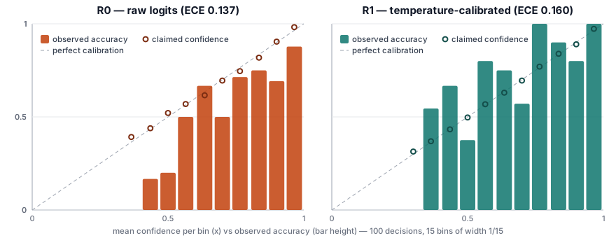
Mean confidence drops from 0.834 to 0.630, and the top of the distribution becomes honest. Five of the seven populated bins above 0.53 now show accuracy at or above confidence; the two exceptions remain mildly overconfident (0.57 accuracy claimed at 0.69 confidence; 0.80 at 0.89). The overconfidence cliff is gone; what remains is a residue, concentrated at the bottom. But here is the finding we didn't expect when we started: global ECE got slightly worse (0.137 → 0.160). The low-confidence tail inverted — seven items now sit at ~31 % confidence with 0 % accuracy — and the 0.47–0.53 bin still runs over (37 % right at 50 % confidence).

The honest lesson: a temperature fitted on one split is a transfer, not a guarantee. It corrects the systematic direction (overconfidence) almost for free, and it provably never changes which option wins: the argmax is invariant under positive scaling, so accuracy stays at 70 % — an invariant the harness asserts on every item. But if your downstream consumer thresholds in the 0.3–0.5 range, a single scalar is not enough; you're in isotonic-regression or bin-wise calibration territory. Calibrate where you act.

R2: blind self-repair — no answer key, 40 % of misses fixed

Now the loop. For each of the 30 misses, we re-render the same prompt with one extra line of feedback — without ever revealing the answer:

Your previous answer was D. That was incorrect. Review the options carefully and answer again.

One more forward pass per miss. Result: 12 of 30 fixed, accuracy 70 % → 82 %. The model's second pass genuinely reconsiders — enough of the probability mass migrates away from the wrong option that the argmax flips in 40 % of cases. No fine-tuning, no gradient, no answer key in the prompt; a strictly local, self-contained correction loop. That is the forecasting analogue of the self-repair we measured for code generation in our companion benchmark: the model contains the information needed to fix itself; the loop just forces a second look at the right altitude.

The 18 that survived blind repair are the interesting residue — look at R1's 0.27–0.33 bin: seven items at ~31 % confidence, 0 % right. The model knows it doesn't know (post-calibration, its low-confidence tail correlates with genuine difficulty). A production agent would abstain or escalate exactly there instead of guessing.

R3: telling the answer is not intelligence

For completeness: feeding the 18 remaining misses the correct option ("the correct answer is A — answer again") fixes all 18, trivially. Accuracy 100 %, but mean confidence drops to 0.727 and ECE rises to 0.273. Corrected models are underconfident — the feedback injects uncertainty even when the model complies. Don't read R3 as capability; read it as instruction-following, and as a reminder that any human-in-the-loop correction loop changes the confidence profile of everything downstream.

Wiring it into an operator agent

The reason we ran this on a laptop GPU rather than in a notebook: the endpoint plugs into predictive-agent-public, our K8s/Docker predictive health monitor. It already had a pluggable LLM analysis layer (Ollama, SAIA, OpenAI-compatible backends) and — crucially — a CalibrationMonitor that tracks predicted-vs-actual outcomes in a rolling window with Brier scoring and drift-triggered rollback. What it didn't have was a backend producing genuinely calibrated probabilities.

The new LLM_BACKEND=jevlocal maps the decision grades onto the operator schema (branch feat/jev-decision-backend in the repo above):

LLMBackend.JEVLOCAL  # POST {question, options} → calibrated probs
# low      → severity=low,    action=Monitor
# moderate → severity=medium, action=Escalate for review
# high     → severity=high,   action=Remediate

with the calibrated distribution attached to every analysis (jev_probabilities, jev_calibrated, jev_confidence). One real request/response pair from the smoke run — the crash-loop incident:

POST /decide
{ "question": "Issue: Pod in CrashLoopBackOff, OOMKilled 14x in 40 min …",
  "options": [ {"id": "low", "text": "Low risk - it will stabilise…"},
               {"id": "moderate", "text": "…"},
               {"id": "high", "text": "High risk - it will keep failing…"} ] }

→ raw P(high) 0.993  →  calibrated P(high) 0.850  →  severity=high, action=Remediate

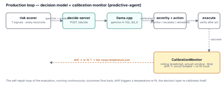
The temperature fit matters precisely at the thresholds the planner acts on: the same call reports raw P = 0.993 against a calibrated 0.850. A healthy pod scores low / monitor at calibrated 0.90. The production self-repair loop is then just CalibrationMonitor doing what R2 did: outcomes flow back, drift triggers a temperature re-fit, the decision layer re-calibrates itself while the circuit breaker keeps blast radius bounded.

Takeaways

1. Raw LLM logits are unusable as probabilities. 13 points of overconfidence, concentrated exactly where consumers trust the number most (≥ 0.93). If you read probabilities off a language model, calibrate first — a fitted temperature is one scalar and five minutes of work.
2. Calibration transfers imperfectly. Our temperature made five of seven bins above 0.53 honest and still worsened global ECE via the low tail. Calibrate in the range where you make decisions; consider isotonic if you act below 0.5.
3. Blind self-repair is real and cheap. One feedback line, no answer key, +12 accuracy points. The misses it can't fix are identifiable — they're the ones the calibrated model flags with low confidence. Abstain there.
4. A decision model is a three-layer architecture, not a product tier: constrained readout, one-scalar calibration, a fixed contract. Everything above is reproducible on a 12 GB GPU with llama.cpp and an afternoon — and the layers are separable enough to swap the base model without touching the consumer.

The full harness lives in graphwiz-jev (scripts/article-experiment.py, branch feat/decide-server), the operator integration on the feat/jev-decision-backend branch of predictive-agent-public — numbers, reliability tables and the raw JSON report included, so you can check our arithmetic.